21  Two Mode Network Analysis

library(igraph)
library(ADAPTSNA)
library(dplyr)

There are many ways to analyse two mode network data. There are some analyses that is done on two mode networks which are very similar to that done on one mode networks with a little twist. Meanwhile, there are some other things that are fairly unique to two mode networks that are fun to play around with. In this chapter, we will cover just two things, centrality and duality in two mode networks. This should be enough to get you comfortable and understanding the fundamental principles of analysing these types of networks.

LEARNING ELEMENTS - Data Discoveries

Degree Centrality in Two Mode Networks

First, let’s go ahead and bring in the Harry Potter data we used so far when working with two mode networks. Here, I use the load_data() call to bring in the adjacency matrix with the group affiliation network for the characters from the fantasy series. Remember, since this is loaded as a .csv, we need to tell R that it is a matrix (meaningful 1s and 0s) before we can use the graph_from_biadjacency_matrix() function to convert it into a network.

hp <- load_data("Harry Potter_Two_Mode_AM.csv", row.names=1)

hp_mat <- as.matrix(hp)

hp_aff <- graph_from_biadjacency_matrix(hp_mat)

Now we have the data ready to go, let’s start with a visual inspection of the network. This is the same visualisation we created when learning about two mode network data. It serves as a reference point for the rest of the analyses we will do here.

shapes <- c("circle", "square") 
colors <-c("green", "orange") 

par(mar =c(5,0,2,0)) 
set.seed(123) 

plot(hp_aff, 
     vertex.color=colors[V(hp_aff)$type+1],
     vertex.shape=shapes[V(hp_aff)$type+1], 
     vertex.label.cex = 0.5, vertex.size = 7, 
     main = "Harry Potter", sub = "Characters Connected to Groups")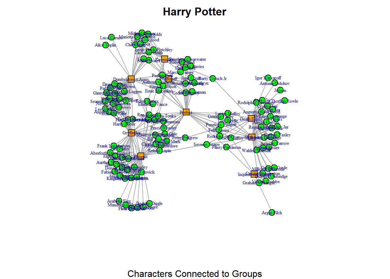

Now let’s turn to some analysis. We have already learned about different measures of centrality, so we won’t go too much into detail here. However, the main thing you must remember when working with centrality in two mode data is that your interpretation of the measures needs to reflect the two mode nature. For the sake of parsimony, we are going to cover degree centrality. S

To get going, we are going to make a quick data frame that captures the degree centrality. We are also going to include the name of each node and an indicator as to whether the node is an character or a group. This is going to come in handy when we are talking about these measures.

centrality <- data.frame(
  degree = degree(hp_aff),
  name = V(hp_aff)$name,
  type = ifelse(V(hp_aff)$type == TRUE, "Group", "Character")
)

The logic of degree centrality remains the same from one mode to two mode analysis. The degree centrality simply counts the number of neighbours that a node has. The important thing to remember, however, is that counting the number of neighbours in a one mode network is usually interpreted as a measure of an indivdual’s prominence in the network. The maximum degree in a one mode network is n-1. When applied to a two mode network, this alters slightly depending on which mode you are measuring. The maximal degree for each mode is the N of the opposite mode.

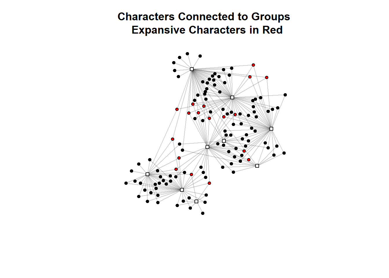
If you are measuring the degree centrality of the individual characters in this network, then what you are actually capturing is the number of groups they belong to. Their maximal degree is the n(groups). While we could still think of this as how prominent a character is within the world Harry Potter, it is more appropriate to think of this as a measure of how expansive they are within this two mode world. The chunk below filters the dataframe we created to focus only on the artists and calculates a brief summary of the their degree centrality.

centrality %>%
  filter(type == "Character") %>%
summarize(mean(degree),
          min = min(degree),
          max = max(degree),
          sd = sd(degree),
          n = n()
          )

  mean(degree) min max        sd   n
1     2.065574   1   4 0.5711769 122

From this, we can infer that the average Character from our set belongs to 2 groups in Harry Potter. However, we can also see from the max and standard deviation that there is some variance among these characters’ expansiveness in terms of their affiliation to groups in the wizarding world. However, the maximum degree is lower than the maximum potential degree (n groups = 9) which suggests that either folk are selective about what groups they are in or there are rules causing people to select in to/out of certain groups (like Hogwarts houses!).

The visualisation below demonstrates the characters with a degree centrality equal to or higher than the average in red while those with below average are black. We do this by adding a vertex characteristic to our graph only for the characters (type = FALSE, groups are set to NA). Groups are left white

V(hp_aff)$character_degree_group <- NA
V(hp_aff)$character_degree_group[V(hp_aff)$type == FALSE] <- 
  ifelse(
    degree(hp_aff, v = V(hp_aff)[V(hp_aff)$type == FALSE]) > 2,
    "Above Avg",
    "Below Avg"
  )

# node shapes
V(hp_aff)$shape <- ifelse(V(hp_aff)$type == FALSE, "circle", "square")

# node colors
V(hp_aff)$color <- ifelse(
  V(hp_aff)$character_degree_group == "Above Avg",
  "red",
  ifelse(
    V(hp_aff)$character_degree_group == "Below Avg",
    "black",
    "grey"
  )
)

set.seed(123)

plot(
  hp_aff,
  layout = layout_with_dh(hp_aff),
  vertex.shape = V(hp_aff)$shape,
  vertex.color = V(hp_aff)$color,
  vertex.size = 4,
  vertex.label = NA,
  edge.arrow.mode = 0,
  edge.color = adjustcolor("black", alpha.f = 0.2),
  main = "Characters Connected to Groups \n Expansive Characters in Red"
)

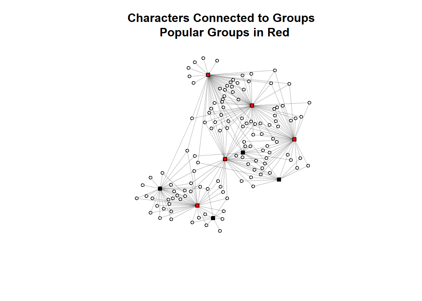
If you are measuring the degree centrality of the second mode, in this case the groups, you are measuring the number of characters that are in each group. As above, the chunk below does the same for groups so that we can compare each.

centrality %>%
  filter(type == "Group") %>%
summarize(mean(degree),
          min = min(degree),
          max = max(degree),
          sd = sd(degree),
          n = n()
          )

  mean(degree) min max       sd n
1           28   9  47 13.14344 9

Here, the average group had roughly 28 characters as members. The standard deviation suggests that there is some variation in this across characters but the observed maximum is much lower than the possible degree (n characters = 122). The visualisation below repeats the aesthetic as above only now showing groups (tpye = TRUE) with a degree above the average.

V(hp_aff)$group_degree_group <- NA
V(hp_aff)$group_degree_group[V(hp_aff)$type == TRUE] <- 
  ifelse(
    degree(hp_aff, v = V(hp_aff)[V(hp_aff)$type == TRUE]) > 28,
    "Above Avg",
    "Below Avg"
  )

# node colors - new rules
V(hp_aff)$color2 <- ifelse(
  V(hp_aff)$group_degree_group == "Above Avg",
  "red",
  ifelse(
    V(hp_aff)$group_degree_group == "Below Avg",
    "black",
    "grey"
  )
)

set.seed(123)

plot(
  hp_aff,
  layout = layout_with_dh(hp_aff),
  vertex.shape = V(hp_aff)$shape,
  vertex.color = V(hp_aff)$color2,
  vertex.size = 4,
  vertex.label = NA,
  edge.arrow.mode = 0,
  edge.color = adjustcolor("black", alpha.f = 0.2),
  main = "Characters Connected to Groups \n Popular Groups in Red"
)

In summary, when working with two mode networks, think about the degree centrality of an individual as a measure of expansiveness within the observed world and the degree of an event as a measure of its popularity (counting the attendees).

Conversion of Two Mode Networks

A second tool for analysing two mode networks converting them to one mode and running further analysis. To do this, you use a method called bipartite projection. Bipartite projection calculates network ties between individuals and groups based on the two mode network. These projections are separated into two networks, one network where individuals are connected to indivduals and second network where groups are connected to groups. Individuals who are both connected to the same group are counted as sharing a tie defined by their mutual affiliation (belonging to the same group). The strength of this tie is weighted by the number of groups they are mutually affiliated with. So, if person A and person B are connected to three of the same groups in the two mode network, then the bipartite projection would calculate a tie between them with a weight (strength) of 3.

The same logic applies to the second mode, the groups. Here, though, the method constructs ties between the groups if they share participants. If group X and group Y share three members, then the strength of their relationship in the projection would be 3.

The chunk below creates a new network object, hp_project, that has both the individual-individual network and the group-group network by using the bipartite_projection() function from igraph. It is structured as a network list with the two types of networks. When you view it, you see the two networks in it - $proj1 and $proj2. proj1 is the network of individuals connected to each other by mutual group affiliation, while proj2 is the network of group to group network. Note that both networks carry the names of the nodes and now an edge characteristics showing the weight of the projected relationship.

hp_project <- bipartite_projection(hp_aff)

hp_project

$proj1
IGRAPH 9f97fb4 UNW- 122 3105 -- 
+ attr: name (v/c), character_degree_group (v/c), shape (v/c), color
| (v/c), group_degree_group (v/c), color2 (v/c), weight (e/n)
+ edges from 9f97fb4 (vertex names):
 [1] Albus Dumbledore--Remus Lupin         
 [2] Albus Dumbledore--Molly Weasley       
 [3] Albus Dumbledore--Siruis Black        
 [4] Albus Dumbledore--Severus Snape       
 [5] Albus Dumbledore--Alastor Moody       
 [6] Albus Dumbledore--Minerva McGonagall  
 [7] Albus Dumbledore--Rubeus Hagrid       
+ ... omitted several edges

$proj2
IGRAPH 9f97fd3 UNW- 9 22 -- 
+ attr: name (v/c), character_degree_group (v/c), shape (v/c), color
| (v/c), group_degree_group (v/c), color2 (v/c), weight (e/n)
+ edges from 9f97fd3 (vertex names):
 [1] Phoenix          --Prefect           Phoenix          --Gryffindor       
 [3] Phoenix          --Death.Eaters      Phoenix          --Slytherin        
 [5] Phoenix          --Hufflepuff        Phoenix          --Ravenclaw        
 [7] Phoenix          --Dumbeldore.s.Army Dumbeldore.s.Army--Prefect          
 [9] Dumbeldore.s.Army--Gryffindor        Dumbeldore.s.Army--Ravenclaw        
[11] Dumbeldore.s.Army--Hufflepuff        Death.Eaters     --Slytherin        
[13] Death.Eaters     --Gryffindor        Death.Eaters     --Prefect          
+ ... omitted several edges

Now, you can analyse these projected networks. Take a look at the visualisations of each. Again, be mindful that the object we have created is a list, so to visualise the network you have to call which of the two (proj1 or proj2). First, we visualise the individuals and then we visualise the groups.

par(mar = c(0,0,2,0))
set.seed(123)
plot(hp_project$proj1, 
     vertex.label = NA, 
     vertex.size = 5, 
     vertex.color = "green", 
     main = "Individual to Individual Projection")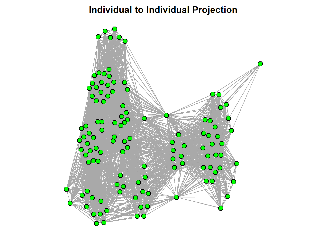

par(mar = c(0,0,2,0))
set.seed(123)
plot(hp_project$proj2, 
     vertex.size = 5, 
     vertex.color = "orange", 
     vertex.shape = "square", 
     main = "Group to Group Projection", 
     edge.width = E(hp_project$proj2)$weight/5)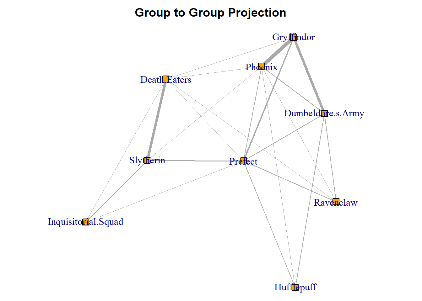

Across both of these projected networks, we can see some fascinating structure of individuals and groups. For instance, look at the group projection network and pay attention to the width of the connections. These suggest that there are some groups that are more closely connected than others. In the individual network, it appears that there are some small clusters or groups that are more closely mutually affiliated to groups than others. From here, you can analyse these one mode projected networks as normal.

Here we have used some fun data and yet revealed some really interesting structures of relationships based on mutual affiliation or shared members. Imagine the utility of this type of analysis to identify groups of individuals connected by TV subscriptions, or shopping behaviours. These would make for some cool marketing analyses!

Summary

In this chapter, you have learned some fundamental methods for analysing two mode networks. This requires you to think specifically about the differences between individuals and groups when considering centrality. Additionally, you can measure the symbolic ways in which individuals are connected to each other or that groups are connected.

Great work!